
Downside risk (safety) mathematics
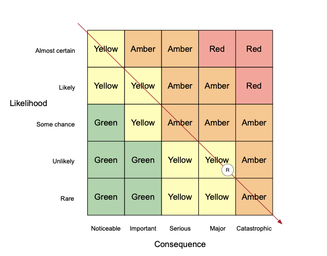
The use of risk curves in the form of risk matrices for acceptable or tolerable risk decision making seems to have made a comeback in recent years. A single point (a dot) is used to characterise the risk associated with a hazard, with the location (red, amber, yellow or green) representing the assessed level of organisational concern.
Most commonly, such a dot represents a point on a line of constant risk on some sort of logarithmic scale. That is, a 10-fold increase in consequence is associated with a 10-fold decrease in likelihood providing for a nominal (diagonal) line of constant risk shown in a typical heat map adjacent. This is really just a logarithmic plot of the positive side of the hyperbolic function y = 1/x.
However, the position that risk is simply a single likelihood x consequence point does not seem to be the way it works at least for engineering risk matters. That is; in order to mathematically describe the risk associated with an engineered circumstance or situation, you need to know the shape of the risk curve associated with that hazard. Failures are rarely just a single point possibility like heads or tails in a coin toss. Lessor outcomes usually have higher frequency but it depends on the nature of the concern. Often it can be a step function especially when considering the possibilities of multiple fatalities.
The cumulative risk associated with any particular hazard is the sum of all the possible risk outcomes which is really what needs to be known. Technically that means integrating the area under the risk curve. Picking just a single point on the risk curve to describe all of the possible outcomes for that hazard is likely to understate the cumulative risk quite significantly.
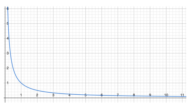
To mathematically demonstrate this, consider the hyperbolic plot shown above. The simple product of likelihood times consequence is 1 anywhere on the line, that is ‘constant risk’. However, the integral from 1 to 10 of y = 1/x is ln(10) – ln(1) or about 2.3. From 1 to 100,000 its 11.51, over an order of magnitude greater than the simple risk product of likelihood x consequence.
This may not matter so much on a relative risk basis, at least for similar consequence levels and thereby as a reporting tool to senior decision makers. But as an absolute value for risk decision making, the simple product of likelihood by consequence for high consequence, low likelihood events are almost certainly in error and should be used with great care. From our perspective, this is why the WHS legislation focuses on control rather than risk, especially for critical (kill or maim) hazards as accurately computing actual risk levels is such a difficult, if near impossible task.